Building Your First Deep Learning Model: A Step-by-Step Guide

Introduction to Deep Learning

Deep learning is a subset of machine learning, which itself is a subset of artificial intelligence (AI). Deep learning models are inspired by the structure and function of the human brain and are composed of layers of artificial neurons. These models are capable of learning complex patterns in data through a process called training, where the model is iteratively adjusted to minimize errors in its predictions.

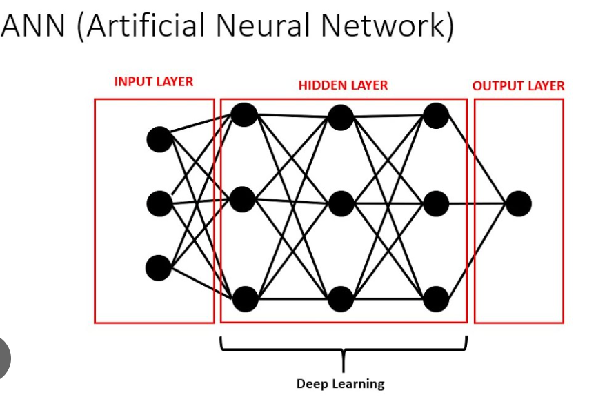
In this blog post, we will walk through the process of building a simple artificial neural network (ANN) to classify handwritten digits using the MNIST dataset.

Understanding the MNIST Dataset

The MNIST dataset (Modified National Institute of Standards and Technology dataset) is one of the most famous datasets in the field of machine learning and computer vision. It consists of 70,000 grayscale images of handwritten digits from 0 to 9, each of size 28x28 pixels. The dataset is divided into a training set of 60,000 images and a test set of 10,000 images. Each image is labeled with the corresponding digit it represents.

Downloading the Dataset

We will use the MNIST dataset provided by the Keras library, which makes it easy to download and use in our model.

Step 1: Importing the Required Libraries

Before we start building our model, we need to import the necessary libraries. These include libraries for data manipulation, visualization, and building our deep learning model.

import numpy as np
import pandas as pd
import matplotlib.pyplot as plt
import seaborn as sns
import tensorflow as tf
from tensorflow import keras

• numpy and pandas are used for numerical and data manipulation.
• matplotlib and seaborn are used for data visualization.
• tensorflow and keras are used for building and training the deep learning model.

Step 2: Loading the Dataset

The MNIST dataset is available directly in the Keras library, making it easy to load and use.

(X_train, y_train), (X_test, y_test) = keras.datasets.mnist.load_data()

This line of code downloads the MNIST dataset and splits it into training and test sets:

• X_train and y_train are the training images and their corresponding labels.
• X_test and y_test are the test images and their corresponding labels.

Step 3: Inspecting the Dataset

Let’s take a look at the shape of our training and test datasets to understand their structure.

print(X_train.shape)
print(X_test.shape)
print(y_train.shape)
print(y_test.shape)

• X_train.shape outputs (60000, 28, 28), indicating there are 60,000 training images, each of size 28x28 pixels.
• X_test.shape outputs (10000, 28, 28), indicating there are 10,000 test images, each of size 28x28 pixels.
• y_train.shape outputs (60000,), indicating there are 60,000 training labels.
• `y_test

.shapeoutputs(10000,)`, indicating there are 10,000 test labels.

To get a better understanding, let’s visualize one of the training images and its corresponding label.

plt.imshow(X_train[2], cmap='gray')
plt.show()
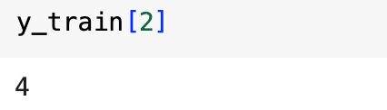
print(y_train[2])

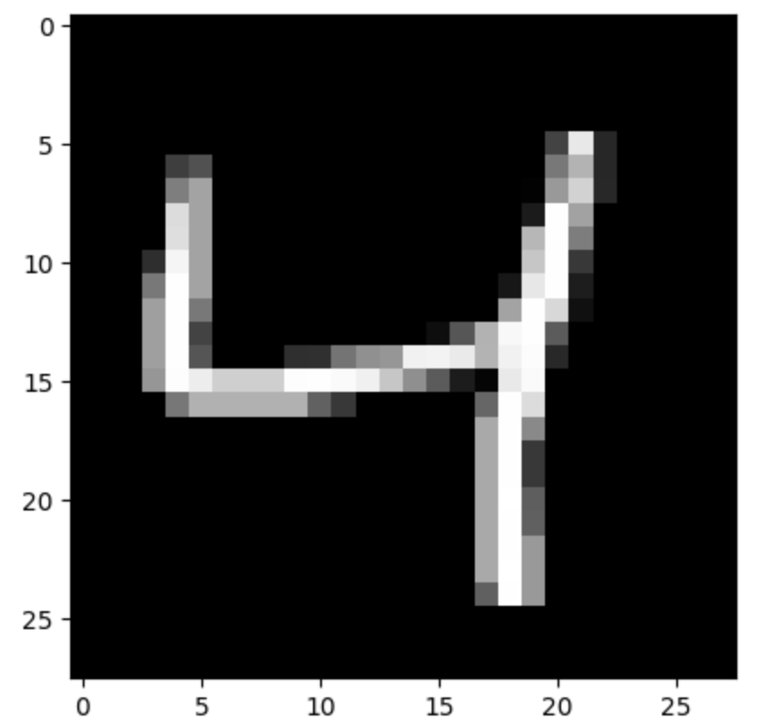
• plt.imshow(X_train[2], cmap='gray') displays the third image in the training set in grayscale.
• plt.show() renders the image.
• print(y_train[2]) outputs the label for the third image, which is the digit the image represents.

Step 4: Rescaling the Dataset

Pixel values in the images range from 0 to 255. To improve the performance of our neural network, we rescale these values to the range [0, 1].

X_train = X_train / 255
X_test = X_test / 255

This normalization helps the neural network learn more efficiently by ensuring that the input values are in a similar range.

Step 5: Reshaping the Dataset

Our neural network expects the input to be a flat vector rather than a 2D image. Therefore, we reshape our training and test datasets accordingly.

X_train = X_train.reshape(len(X_train), 28 * 28)
X_test = X_test.reshape(len(X_test), 28 * 28)

• X_train.reshape(len(X_train), 28 * 28) reshapes the training set from (60000, 28, 28) to (60000, 784), flattening each 28x28 image into a 784-dimensional vector.
• Similarly, X_test.reshape(len(X_test), 28 * 28) reshapes the test set from (10000, 28, 28) to (10000, 784).

Step 6: Building Our First ANN Model

We will build a simple neural network with one input layer and one output layer. The input layer will have 784 neurons (one for each pixel), and the output layer will have 10 neurons (one for each digit).

ANN1 = keras.Sequential([
    keras.layers.Dense(10, input_shape=(784,), activation='sigmoid')
])

• keras.Sequential() creates a sequential model, which is a linear stack of layers.
• keras.layers.Dense(10, input_shape=(784,), activation='sigmoid') adds a dense (fully connected) layer with 10 neurons, input shape of 784, and sigmoid activation function.

Next, we compile our model by specifying the optimizer, loss function, and metrics.

ANN1.compile(optimizer='adam', loss='sparse_categorical_crossentropy', metrics=['accuracy'])

• optimizer='adam' specifies the Adam optimizer, which is an adaptive learning rate optimization algorithm.
• loss='sparse_categorical_crossentropy' specifies the loss function, which is suitable for multi-class classification problems.
• metrics=['accuracy'] specifies that we want to track accuracy during training.

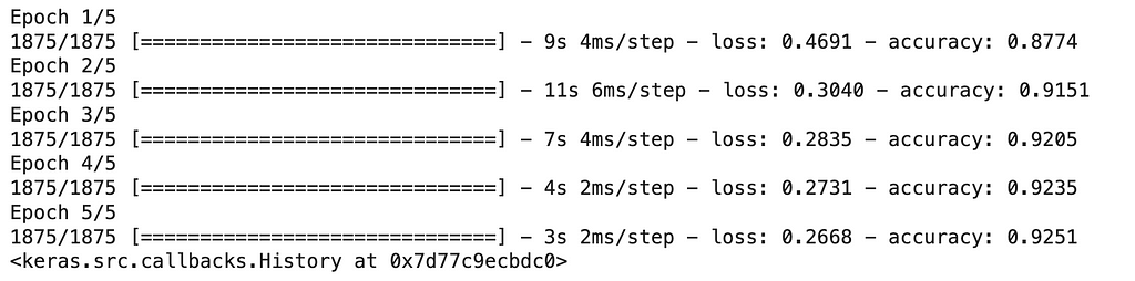
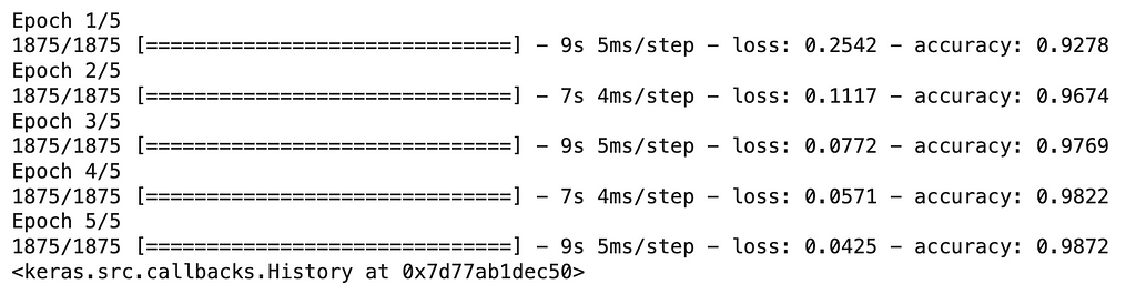
We then train the model on the training data.

ANN1.fit(X_train, y_train, epochs=5)

• ANN1.fit(X_train, y_train, epochs=5) trains the model for 5 epochs. An epoch is one complete pass through the training data.

Step 7: Evaluating the Model

After training the model, we evaluate its performance on the test data.

ANN1.evaluate(X_test, y_test)

• ANN1.evaluate(X_test, y_test) evaluates the model on the test data and returns the loss value and metrics specified during compilation.

Step 8: Making Predictions

We can use our trained model to make predictions on the test data.

y_predicted = ANN1.predict(X_test)

• ANN1.predict(X_test) generates predictions for the test images.

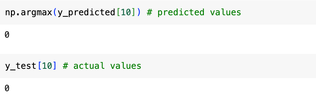
To see the predicted label for the first test image:

print(np.argmax(y_predicted[10]))
print(y_test[10])

• np.argmax(y_predicted[10]) returns the index of the highest value in the prediction vector, which corresponds to the predicted digit.
• print(y_test[10]) prints the actual label of the first test image for comparison.

Step 9: Building a More Complex ANN Model

To improve our model, we add a hidden layer with 150 neurons and use the ReLU activation function, which often performs better in deep learning models.

ANN2 = keras.Sequential([
    keras.layers.Dense(150, input_shape=(784,), activation='relu'),
    keras.layers.Dense(10, activation='sigmoid')
])

• keras.layers.Dense(150, input_shape=(784,), activation='relu') adds a dense hidden layer with 150 neurons and ReLU activation function.

We compile and train the improved model in the same way.

ANN2.compile(optimizer='adam', loss='sparse_categorical_crossentropy', metrics=['accuracy'])
ANN2.fit(X_train, y_train, epochs=5)

Step 10: Evaluating the Improved Model

We evaluate the performance of our improved model on the test data.

ANN2.evaluate(X_test, y_test)

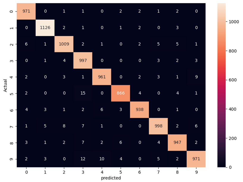
Step 11: Confusion Matrix

To get a better understanding of how our model performs, we can create a confusion matrix.

y_predicted2 = ANN2.predict(X_test)
y_predicted_labels2 = [np.argmax(i) for i in y_predicted2]

• y_predicted2 = ANN2.predict(X_test) generates predictions for the test images.
• y_predicted_labels2 = [np.argmax(i) for i in y_predicted2] converts the prediction vectors to label indices.

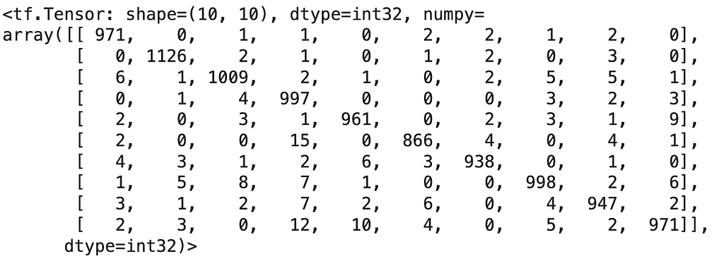
We then create the confusion matrix and visualize it.

cm = tf.math.confusion_matrix(labels=y_test, predictions=y_predicted_labels2)

plt.figure(figsize=(10, 7))
sns.heatmap(cm, annot=True, fmt='d')
plt.xlabel("Predicted")
plt.ylabel("Actual")
plt.show()

• tf.math.confusion_matrix(labels=y_test, predictions=y_predicted_labels2) generates the confusion matrix.
• sns.heatmap(cm, annot=True, fmt='d') visualizes the confusion matrix with annotations.

Conclusion

In this blog post, we covered the basics of deep learning and walked through the steps of building, training, and evaluating a simple ANN model using the MNIST dataset. We also improved the model by adding a hidden layer and using a different activation function. Deep learning models, though seemingly complex, can be built and understood step-by-step, enabling us to tackle various machine learning problems.

This brings us to the end of this article. I hope you have understood everything clearly. Make sure you practice as much as possible.

If you wish to check out more resources related to Data Science, Machine Learning and Deep Learning you can refer to my Github account.

You can connect with me on LinkedIn — RAVJOT SINGH.

I hope you like my article. From a future perspective, you can try other algorithms also, or choose different values of parameters to improve the accuracy even further. Please feel free to share your thoughts and ideas.

P.S. Claps and follows are highly appreciated.

Building Your First Deep Learning Model: A Step-by-Step Guide was originally published in Becoming Human: Artificial Intelligence Magazine on Medium, where people are continuing the conversation by highlighting and responding to this story.